Web Scraping Episodes from Scientific American’s Podcast
Published:
In this blog post, I will walk you through the process of scraping episode information from the Science Quickly Podcast, available at Scientific American’s website. This project aims to retrieve essential details about each episode, and provide insight into the topics discussed by the podcast since its relaunch.
The data will be saved in a CSV file for further analysis.
1. Setting Up
Importing Library Packages
To get started, we need to import the necessary libraries. We will use pandas for data manipulation and selenium for web scraping.
import pandas as pd
from selenium import webdriver
from selenium.webdriver.firefox.service import Service
from selenium.webdriver.common.by import By
from selenium.webdriver.firefox.options import Options
import time

# Set Firefox options (optional, for example, headless mode)
options = Options()
options.headless = True  # Optional, set True for headless mode

# Create a Service object to specify the geckodriver path
service = Service("/Users/julieliu/geckodriver")  # Adjust the path to your geckodriver
2. Starting the Scraping Process
This step will take approximately 4 minutes.
Initialize the WebDriver
We will initialize the WebDriver and generate a list of URLs for pages 1 to 50 of the podcast episodes.
# Initialize the WebDriver
driver = webdriver.Firefox(service=service, options=options)

# Generate the list of URLs for pages 1 to 50
url_list = [f"https://www.scientificamerican.com/podcast/science-quickly/?page={i}" for i in range(1, 51)]

# Create a list to store the extracted information
data = []

# Loop through each URL
for url in url_list:
    try:
        # Visit the page
        driver.get(url)
        print(f"Scraping URL: {url}")

        # Allow some time for the page to load
        driver.implicitly_wait(5)

        # Find all articles representing episodes on the page
        episodes = driver.find_elements(By.CSS_SELECTOR, 'article.article-pFLe7')

        # Loop through each episode and extract the information
        for episode in episodes:
            try:
                # Extract the title
                title_element = episode.find_element(By.CSS_SELECTOR, 'h2.articleTitle-mtY5p')
                title = title_element.text

                # Extract the summary
                summary_element = episode.find_element(By.CSS_SELECTOR, 'div.dek-KweYs p')
                summary = summary_element.text

                # Extract the authors
                author_element = episode.find_element(By.CSS_SELECTOR, 'p.authors-NCGt1')
                authors = author_element.text

                # Extract the category (e.g., "Spacecraft")
                category_element = episode.find_element(By.CSS_SELECTOR, 'div.kicker-EEaW-')
                category = category_element.text.split('\n')[0]  # Take only the first line

                # Extract the date (e.g., "September 13, 2024")
                date_element = episode.find_element(By.CSS_SELECTOR, 'span.kickerMeta-0zV3t')
                date = date_element.text

                # Append the data as a dictionary to the list
                data.append({
                    "Title": title,
                    "Date": date,
                    "Category": category,
                    "Summary": summary,
                    "Authors": authors
                })

            except Exception as e:
                print(f"Error extracting episode: {e}")

        # Pause for a short time to avoid overwhelming the server
        time.sleep(2)

    except Exception as e:
        print(f"Error scraping page {url}: {e}")

# Close the browser
driver.quit()
3. Storing the Results
Finally, we will convert the list of dictionaries to a pandas DataFrame and save it as a CSV file.
# Convert the list of dictionaries to a pandas DataFrame
df = pd.DataFrame(data)

# Save the DataFrame to a CSV file
df.to_csv("podcast_episodes.csv", index=False)

# Print the DataFrame
print(df)
4. Visualization of Categories
Data Cleaning
- Filter out data after May 3rd, 2024.
- Since there are many categories and some of them are similar to each other. We can map categories to broader ones.
import matplotlib.pyplot as plt
import seaborn as sns
import pandas as pd

# Read the CSV file
df = pd.read_csv("podcast_episodes.csv")

# Turn category into lower case with first letter capital
df['Category'] = df['Category'].str.title()

# Exclude year 2019
df = df[df['Date'].str.contains('2019') == False]

df.head()
# Read the CSV file
df = pd.read_csv("podcast_episodes.csv")

# Turn category into lower case with first letter capital
df['Category'] = df['Category'].str.title()

# Extract data after May 3rd, 2024 (this is the relaunch date of the podcast)
df['Date'] = pd.to_datetime(df['Date'])
df = df[df['Date'].dt.strftime('%Y-%m-%d') >= '2024-05-03']

df.head()
# List out all the categories
category = df['Category'].unique()
print(category)

# Remove "September 18, 2024" category
df = df[df['Category'] != 'September 18, 2024']

# Define new categories
# We have AI and Technology, Social Science, Climate and Environment,
# Health and Wellness, and Space Science

# Create a dictionary to map the old categories to the new categories
category_mapping = {
    'Math': 'Mathematics',
    'Medicine': 'Health and Medicine',
    'Technology': 'Technology and AI',
    'Health Care': 'Health and Medicine',
    'Public Health': 'Health and Medicine',
    'Artificial Intelligence': 'Technology and AI',
    'Spacecraft': 'Space and Astronomy',
    'Space & Physics': 'Space and Astronomy',
    'Space Exploration': 'Space and Astronomy',
    'Aging': 'Health and Medicine',
    'Plants': 'Life Sciences',
    'Social Sciences': 'Social Sciences',
    'Oceans': 'Earth and Environment',
    'Environment': 'Earth and Environment',
    'Archaeology': 'Social Sciences',
    'Health': 'Health and Medicine',
    'Neuroscience': 'Life Sciences',
    'Climate Change': 'Earth and Environment',
    'Animals': 'Life Sciences',
    'Fossil Fuels': 'Earth and Environment',
    'Weather': 'Earth and Environment',
    'Nuclear Weapons': 'Technology and AI',
    'Food': 'Life Sciences',
    'Conservation': 'Earth and Environment',
    'Marijuana': 'Health and Medicine',
    'Culture': 'Social Sciences'
}

# Apply the mapping to create a new 'Broad Category' column
df['Broad Category'] = df['Category'].map(category_mapping)

# Print unique category and broad category
print("\nUnique categories after mapping and cleaning:")
print(df['Category'].unique())
print("\nUnique broad categories after mapping and cleaning:")
print(df['Broad Category'].unique())

# Print unique pair of category and broad category sorted by broad category
print(df[['Category', 'Broad Category']].drop_duplicates().sort_values(by='Broad Category'))

# Calculate number of categories
broad_category = df['Broad Category'].unique()
print(broad_category)
Visualization
# Define the color mapping based on the image
color_mapping = {
'Health and Medicine': '#8CD17D',
'Earth and Environment': '#F1A340',
'Mathematics and Physics': '#A6CEE3',
'Space and Astronomy': '#E78AC3',
'Social Sciences': '#B2DF8A',
'Technology and AI': '#FFD92F',
'Life Sciences': '#DFC27D'
}
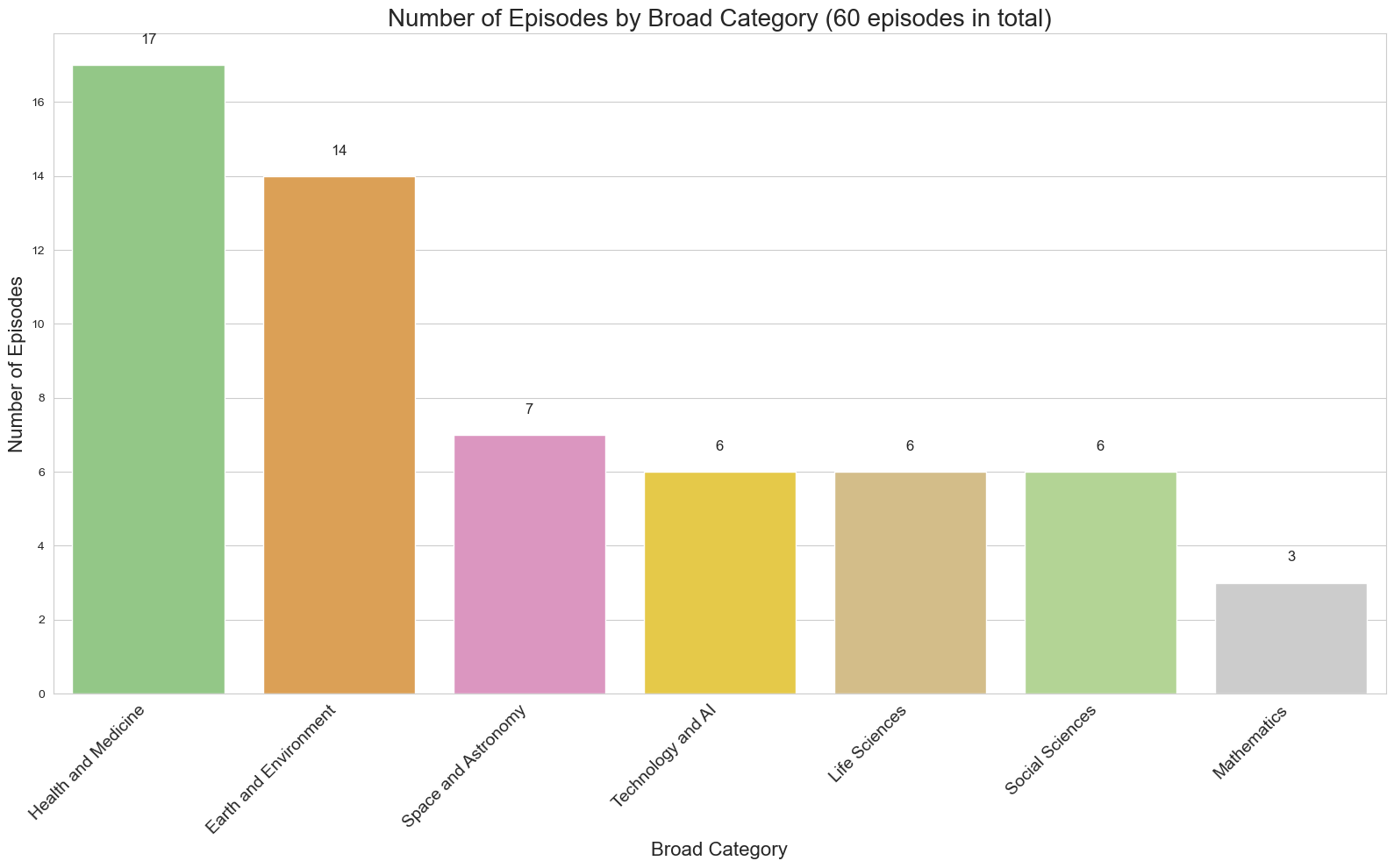
# Count the number of episodes per broad category
broad_category_counts = df['Broad Category'].value_counts()
# Sort the categories by count in descending order
broad_category_counts_sorted = broad_category_counts.sort_values(ascending=False)
# Create a list of colors in the same order as the sorted categories
colors = [color_mapping.get(cat, '#CCCCCC') for cat in broad_category_counts_sorted.index]
# Create the bar chart
plt.figure(figsize=(16, 10))
sns.set_style("whitegrid")
ax = sns.barplot(x=broad_category_counts_sorted.index, y=broad_category_counts_sorted.values, palette=colors)
plt.title('Number of Episodes by Broad Category (60 episodes in total)', fontsize=20)
plt.xlabel('Broad Category', fontsize=16)
plt.ylabel('Number of Episodes', fontsize=16)
plt.xticks(rotation=45, ha='right', fontsize=14)
# Add value labels on top of each bar
for i, v in enumerate(broad_category_counts_sorted.values):
ax.text(i, v + 0.5, str(v), ha='center', va='bottom', fontsize=12)
plt.tight_layout()
plt.show()
# Print the total number of broad categories
print(f"Total number of broad categories: {len(broad_category_counts)}")
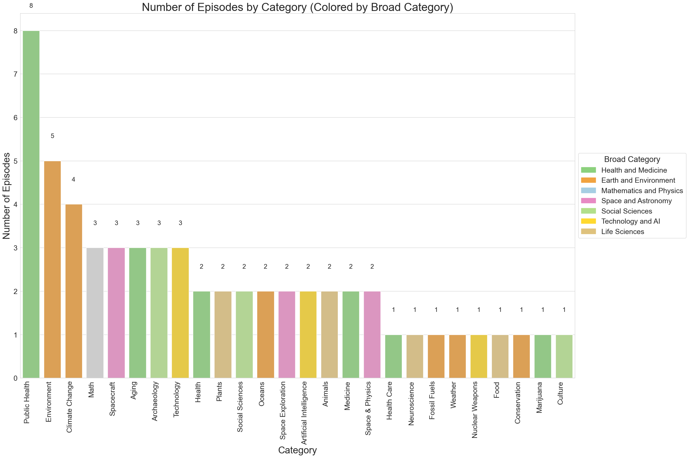
Additional Visualization
# Count the number of episodes per category
category_counts = df['Category'].value_counts()

# Sort the categories by count in descending order
category_counts_sorted = category_counts.sort_values(ascending=False)

# Create a DataFrame with category counts and their broad categories
category_data = pd.DataFrame({
    'Category': category_counts_sorted.index,
    'Count': category_counts_sorted.values,
    'Broad Category': [category_mapping.get(cat, 'Other') for cat in category_counts_sorted.index]
})

# Create the bar chart
plt.figure(figsize=(24, 16))
sns.set_style("whitegrid")

ax = sns.barplot(x='Category', y='Count', data=category_data,
                 palette=[color_mapping.get(bc, '#CCCCCC') for bc in category_data['Broad Category']])

plt.title('Number of Episodes by Category (Colored by Broad Category)', fontsize=28)
plt.xlabel('Category', fontsize=24)
plt.ylabel('Number of Episodes', fontsize=24)
plt.xticks(rotation=90, ha='right', fontsize=18)
plt.yticks(fontsize=18)

# Add value labels on top of each bar
for i, v in enumerate(category_data['Count']):
    ax.text(i, v + 0.5, str(v), ha='center', va='bottom', fontsize=16)

# Add a legend for broad categories
handles = [plt.Rectangle((0,0),1,1, color=color_mapping[label]) for label in color_mapping.keys()]
plt.legend(handles, color_mapping.keys(), title='Broad Category',
           loc='center left', bbox_to_anchor=(1, 0.5), fontsize=18, title_fontsize=20)

plt.tight_layout()
plt.show()

# Print the total number of categories
print(f"Total number of categories: {len(category_counts)}")